The Butterfly Algorithm
Danny Hermes (dhermes)

February 11, 2015
You can find the source of these slides on GitHub.
%matplotlib inline
from make_partition_plots import make_butterfly
make_butterfly()

Outline
- Background for Butterfly
- Motivation from DFT
- Details of Algorithm and Speedup
- Code and Comparison
Setting the Stage
$$\widehat{f}(\xi) = \mathcal{F}f(\xi) = \int_{\mathbb{R}} \text{exp}\left(- 2 \pi x \xi \sqrt{-1}\right) f(x) \, dx$$
$$\widehat{f}_k = \sum_{j = 0}^{N - 1} \text{exp}\left(- \frac{2 \pi k j \sqrt{-1}}{N}\right) f_j$$
from IPython import display

display.Audio(filename='resources/bluewhale.wav')
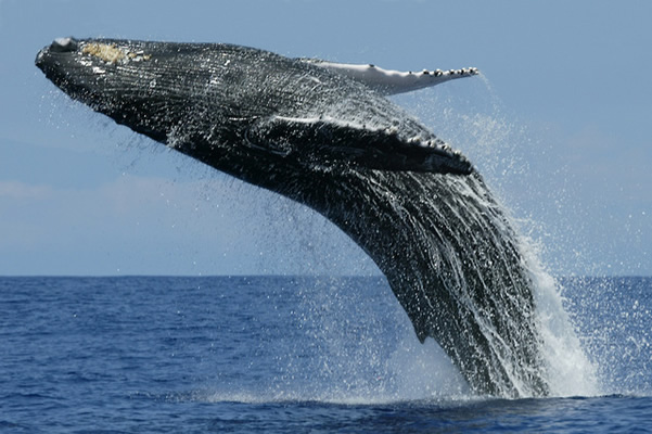
sampling_rate, blue_whale_call = load_whale()

N = len(blue_whale_call)
time_base = np.arange(N) * 10.0 / sampling_rate
from matplotlib import pyplot as plt


plt.plot(time_base, blue_whale_call)
plt.title('Blue Whale B Call')
plt.xlim((time_base[0], time_base[-1]))
plt.xlabel('Time (seconds)')
plt.ylabel('Amplitude')
plt.show()

import time


start = time.time()
dft_whale_call = np.fft.fft(blue_whale_call, n=N)
fft_duration = time.time() - start

message = r'\text{Duration with FFT optimized: } %2.10f' % (fft_duration,)
display.display(display.Math(message))
re_sampled_time = np.arange(len(dft_whale_call)) * sampling_rate / (10.0 * N)
amplitude = np.abs(dft_whale_call) / N

plt.plot(re_sampled_time[:N/2], amplitude[:N/2])

plt.xlabel('Frequency (Hz)')
plt.ylabel('Amplitude')
plt.title('Component Frequencies')
plt.show()

From DFT to Butterflies
$$\widehat{f}_k = \sum_{j = 0}^{N - 1} K(t_k, s_j) \, f_j$$
from make_partition_plots import get_random_intervals
from make_partition_plots import naive_interaction


S_VALUES, T_VALUES = get_random_intervals(16)
naive_interaction(S_VALUES, T_VALUES, N=16)

$$\widehat{f}(t) = \sum_{s} K(t, s) \, D(s)$$
DFT as Butterfly
$$t_k = 2 \pi k, \quad s_j = \frac{j}{N}, \quad K(t, s) = e^{- t s \sqrt{-1}}$$
Naive gets Quadratic
We see that in the most naive implementation, the runtime is quadratic.
def compute_f_hat(f, t, s, kernel_func):
    f_hat = np.zeros(f.shape, dtype=np.complex128)
    for k in xrange(len(f)):
        # Vectorized update.
        f_hat[k] = np.sum(kernel_func(t[k], s) * f)

    return f_hat
# We expect a "slowdown factor" of N / log N
expected_quadratic = fft_duration * N / np.log2(N)

message = r'\text{Expected Quadratic Run-time: } %2.10f' % (expected_quadratic,)
display.display(display.Math(message))
N_vals = np.arange(N, dtype=np.float64)
t = 2 * np.pi * N_vals
s = N_vals / N


def dft_kernel(t, s):
    return np.exp(- 1.0j * t * s)


start = time.time()
f_hat = compute_f_hat(blue_whale_call, t, s, dft_kernel)
naive_duration = time.time() - start

message = r'\text{Actual Naive Duration: } %2.10f' % (naive_duration,)
display.display(display.Math(message))
Is the naive implementation correct?
error = np.linalg.norm(f_hat - dft_whale_call, ord=2)

sig, exponent = str(error).split('e')
expr = r'\|e\|_2 = %s \cdot 10^{%s}' % (sig, exponent)
display.display(display.Math(expr))
Doing Better than Quadratic
naive_interaction(S_VALUES, T_VALUES, N=16)
from make_partition_plots import binned_interaction
binned_interaction(S_VALUES, T_VALUES, L=2)

$$\widehat{f}(t) = \sum_{s} K(t, s) \, D(s) \approx \sum_{\widehat{s}} K' \left(t, \widehat{s}\right) D\left(\widehat{s}\right)$$
$$\mathbf{\text{DFT: }} s_j = \frac{j}{N} \in \left[0, 1\right), \quad 2^L \text{ segments} \Longrightarrow \sigma_{j} = \frac{2j + 1}{2^{L + 1}}$$
from make_partition_plots import make_1D_centers
make_1D_centers(L=2, s_values=S_VALUES)

$$K(t, s) = e^{- t s \sqrt{-1}}, \, ts = t \sigma + t (s - \sigma) \Longrightarrow K(t, s) = K(t, \sigma) K(t, s - \sigma)$$
$$\widehat{f}(t) = \sum_{\sigma} K(t, \sigma) \left[\sum_{s \in B(\sigma)} K(t, s - \sigma) D(s)\right]$$
$$\widehat{f}(t) = \sum_{\sigma} K(t, \sigma) \underbrace{\left[\sum_{s \in B(\sigma)} K(t, s - \sigma) D(s)\right]}_{D(\sigma)}$$
$$\widehat{f}(t) = \sum_{\sigma} K(t, \sigma) D(\sigma)$$
Operation Count
$$2^L \text{ boxes}, \quad 2^L = \mathcal{O}\left(N\right), \quad \left|B(\sigma)\right| = \mathcal{O}(1)$$
$$\begin{align*} \sum_{s \in B(\sigma)} K(t, s - \sigma) D(s) &\rightarrow \mathcal{O}(1) \\ \widehat{f}_k &\rightarrow \mathcal{O}(N) \\ \widehat{f} &\rightarrow \mathcal{O}\left(N^2\right). \end{align*}$$
But We Want Better Than Quadratic
$$K(t, s) \approx \sum_{\alpha = 0}^{M - 1} T_{\alpha}(t) S_{\alpha}(s)$$
$$\text{exp}\left(- t s \sqrt{-1}\right) \approx \sum_{\alpha = 0}^{M - 1} \frac{\left(- \sqrt{-1}\right)^{\alpha}}{\alpha!} t^{\alpha} s^{\alpha}$$
$$\widehat{f}(t) \approx \sum_{\sigma} K(t, \sigma) \sum_{s \in B(\sigma)} \sum_{\alpha = 0}^{M - 1} \frac{\left(- \sqrt{-1}\right)^{\alpha}}{\alpha!} t^{\alpha} \left(s - \sigma\right)^{\alpha} D(s)$$
$$K'(t, \sigma, \alpha) = K(t, \sigma) t^{\alpha}, \quad D(\sigma, \alpha) = \sum_{s \in B(\sigma)} \frac{\left(- \sqrt{-1}\right)^{\alpha}}{\alpha!} \left(s - \sigma\right)^{\alpha} D(s)$$
$$\widehat{f}(t) = \sum_{\sigma, \alpha} K'(t, \sigma, \alpha) D(\sigma, \alpha)$$
$$K(t, s - \sigma) \approx \sum_{\alpha = 0}^{M - 1} \frac{\left(- \sqrt{-1}\right)^{\alpha}}{\alpha!} t^{\alpha} \left(s - \sigma\right)^{\alpha} \text{ when } \left|t\right| \gg 1$$
$$K(t - \tau, s - \sigma) \approx \sum_{\alpha = 0}^{M - 1} \frac{\left(- \sqrt{-1}\right)^{\alpha}}{\alpha!} (t - \tau)^{\alpha} \left(s - \sigma\right)^{\alpha} \text{ for } t \in B(\tau)$$
$$\left|(t - \tau)(s - \sigma)\right| \leq r_{\tau} r_{\sigma} \text{ uniformly bounded}$$
Partitioning the Inputs
- $\mathbb{R}$: binary tree
- $\mathbb{R}^2$ / $\mathbb{C}$: quadtree
- $\mathbb{R}^k$: k-d tree
make_butterfly(L=4, level=0)

make_butterfly(L=4, level=1)

make_butterfly(L=4, level=2)

make_butterfly(L=4, level=3)

make_butterfly(L=4, level=4)

$$\left|(t - \tau)(s - \sigma)\right| \leq r_{\tau} r_{\sigma} \text{ uniformly bounded}$$
$$K(t - \tau, s - \sigma)$$
$$\widehat{f}(t) \approx \sum_{\sigma} K(t, \sigma) \sum_{s \in B(\sigma)} \sum_{\alpha = 0}^{M - 1} \frac{\left(- \sqrt{-1}\right)^{\alpha}}{\alpha!} t^{\alpha} \left(s - \sigma\right)^{\alpha} D(s) \text{ when } \left|t\right| \gg 1$$
$$\widehat{f}(t) \approx \sum_{\sigma} \cdots \sum_{s \in B(\sigma)} \sum_{\alpha = 0}^{M - 1} \frac{\left(- \sqrt{-1}\right)^{\alpha}}{\alpha!} (t - \tau)^{\alpha} \left(s - \sigma\right)^{\alpha} D(s)$$
import sympy


t, s, tau, sigma = sympy.symbols('t s tau sigma')
RHS = tau * sigma + tau * (s - sigma) + sigma * (t - tau) + (s - sigma) * (t - tau)
display.display(display.Math(sympy.latex(RHS)))
display.display(display.Math(sympy.latex(RHS.simplify())))
$$K(t, s) = K(\tau, \sigma) K(t - \tau, \sigma) K(\tau, s - \sigma) K(t - \tau, s - \sigma)$$
$$K(t, s) \approx K(\tau, \sigma) K(t - \tau, \sigma) K(\tau, s - \sigma) \sum_{\alpha = 0}^{M - 1} \frac{\left(- \sqrt{-1}\right)^{\alpha}}{\alpha!} (t - \tau)^{\alpha} \left(s - \sigma\right)^{\alpha}$$
$$K'(t, \sigma, \alpha) = K(t - \tau, \sigma) (t - \tau)^{\alpha}$$
$$D(\tau, \sigma, \alpha) = \frac{\left(- \sqrt{-1}\right)^{\alpha}}{\alpha!} K(\tau, \sigma) \sum_{s \in B(\sigma)} K(\tau, s - \sigma) \left(s - \sigma\right)^{\alpha} D(s)$$
$$\widehat{f}(t) = \sum_{\sigma, \alpha} K'(t, \sigma, \alpha) D(\tau, \sigma, \alpha)$$
Are we there yet?
Computing $D\left(\tau, \sigma, \alpha\right)$
- $M$ choices of $\alpha$
- $2^{\ell}$ choices of $\tau$
- $2^{L - \ell}$ choices of $\sigma$
In total: $M \cdot 2^L = \mathcal{O}\left(N\right)$
We start with $\ell = 0$ and consider what it might take to compute.
make_butterfly(L=4, level=0)
Counting Operations: $\ell = 0$
• $\left|\left\{B(\tau)\right\}_{\tau}\right| = 1$
• $\left|\left\{B(\sigma)\right\}_{\sigma}\right| = 2^L = \mathcal{O}(N)$
• $\left|\left\{D(\tau, \sigma, \alpha)\right\}_{\tau, \sigma, \alpha}\right| = \mathcal{O}(N)$
• $\widehat{f}(t) = \displaystyle \sum_{\sigma, \alpha} K'(t, \sigma, \alpha) D(\tau, \sigma, \alpha)$ takes $\mathcal{O}(N)$
• Total: $\mathcal{O}\left(N^2\right)$ since $D(\tau, \sigma, \alpha) = \displaystyle \sum_{s \in B(\sigma)} \cdots$
Instead we consider the end where $\ell = L$.
make_butterfly(L=4, level=4)
Counting Operations: $\ell = L$
• $\left|\left\{B(\tau)\right\}_{\tau}\right| = 2^L = \mathcal{O}(N)$
• $\left|\left\{B(\sigma)\right\}_{\sigma}\right| = 1$
• $\widehat{f}(t) = \displaystyle \sum_{\sigma, \alpha} K'(t, \sigma, \alpha) D(\tau, \sigma, \alpha)$ takes $\mathcal{O}(1)$
• Now $D(\tau, \sigma, \alpha) = \displaystyle \sum_{s \in B(\sigma)} \cdots$ is $\mathcal{O}(N)$
• Total: still $\mathcal{O}\left(N^2\right)$
Takeaway
$$\ell = 0 \Longrightarrow \sum_{s \in B(\sigma)} \text{ is cheap } \Longrightarrow D(\tau, \sigma, \alpha) \text{ is cheap}$$
$$\ell = L \Longrightarrow \sum_{\sigma, \alpha} \text{ is cheap } \Longrightarrow \widehat{f}(t) \text{ is cheap}$$
Now What
$$\left\{D(\tau, \sigma, \alpha)\right\}_{\ell = 0} \rightarrow \cdots \rightarrow \left\{D(\tau, \sigma, \alpha)\right\}_{\ell = L}$$
$$D(\tau, \sigma, \alpha) = \frac{1}{\alpha!} \sum_{s \in B(\sigma)} K(\tau, s) \left(-\sqrt{-1}\right)^{\alpha} (s - \sigma)^{\alpha} D(s)$$
$$W = \frac{\max(s) - \min(s)}{2^{L - \ell}}$$
$$\left[\begin{matrix} s_0 \\ s_1 \\ \vdots \\ s_{N - 1} \end{matrix}\right] \mapsto \left[\begin{matrix} \left\lfloor\frac{s_0 - \min(s)}{W}\right\rfloor \\ \left\lfloor\frac{s_1 - \min(s)}{W}\right\rfloor \\ \vdots \\ \left\lfloor\frac{s_{N - 1} - \min(s)}{W}\right\rfloor \end{matrix}\right] = \left[\begin{matrix} b_0 \\ b_1 \\ \vdots \\ b_{N - 1} \end{matrix}\right] \mapsto \left[\begin{matrix} \sigma_0 + b_0 W \\ \sigma_0 + b_1 W \\ \vdots \\ \sigma_0 + b_{N - 1} W \end{matrix}\right]$$
def get_bins_and_deltas(vals, min_val, bin_width, num_bins):
    bin_indices = np.floor((vals - min_val) / bin_width)
    # max(vals) falls in the last bin
    bin_indices = np.minimum(bin_indices, num_bins - 1)

    bin_centers = min_val + (0.5 + bin_indices) * bin_width
    return bin_indices.astype(int), vals - bin_centers
$$D(\tau, \sigma, \alpha) = \frac{1}{\alpha!} \sum_{s \in B(\sigma)} K(\tau, s) \left(-\sqrt{-1}\right)^{\alpha} (s - \sigma)^{\alpha} D(s)$$
$$\left[\begin{matrix} s_0 \\ s_1 \\ \vdots \\ s_{N - 1} \end{matrix}\right] \mapsto \left[\begin{matrix} s_0 - \sigma(s_0) \\ s_1 - \sigma(s_1) \\ \vdots \\ s_{N - 1} - \sigma\left(s_{N - 1}\right) \end{matrix}\right] = \left[\begin{matrix} d_0 \\ d_1 \\ \vdots \\ d_{N - 1} \end{matrix}\right] \mapsto \left[\begin{matrix} d_0^0 & d_0^1 & \cdots & d_0^{M - 1} \\ d_1^0 & d_1^1 & \cdots & d_1^{M - 1} \\ \vdots & \vdots & \ddots & \vdots \\ d_{N - 1}^0 & d_{N - 1}^1 & \cdots & d_{N - 1}^{M - 1} \end{matrix}\right]$$
def create_initial_data(s_values, min_s, max_s, tau,
                        actual_data, num_bins, M):
    bin_width = (max_s - min_s) / float(num_bins)
    bin_indices, s_deltas = get_bins_and_deltas(s_values, min_s,
                                                bin_width, num_bins)

    sum_parts = np.zeros((len(s_values), M), dtype=np.complex128)
    sum_parts[:, 0] = dft_kernel(tau, s_values) * actual_data

    for alpha in xrange(1, M):
        sum_parts[:, alpha] = (sum_parts[:, alpha - 1] * s_deltas *
                               (-1.0j) / alpha)

    result = []
    curr_sigma = min_s + 0.5 * bin_width
    for bin_index in xrange(num_bins):
        sum_across_bin = np.sum(
            sum_parts[np.where(bin_indices == bin_index)[0], :], axis=0)
        result.append((tau, curr_sigma, sum_across_bin.reshape(M, 1)))
        curr_sigma += bin_width

    return result
$$\cdots \rightarrow \left\{D(\tau, \sigma, \alpha)\right\}_{\ell = L}$$
$$\widehat{f}(t) = \sum_{\sigma, \alpha} K(t - \tau, \sigma) \left(t - \tau\right)^{\alpha} D(\tau, \sigma, \alpha)$$
$$d_k = t_k - \tau(t_k)$$
$$\left[\begin{matrix} d_0^0 & \cdots & d_0^{M - 1} \\ \vdots & \ddots & \vdots \\ d_{N - 1}^0 & \cdots & d_{N - 1}^{M - 1} \end{matrix}\right] \otimes \left[\begin{matrix} D\left(\tau(t_0), \sigma, 0\right) & \cdots & D\left(\tau(t_0), \sigma, M - 1\right) \\ \vdots & \ddots & \vdots \\ D\left(\tau(t_{N - 1}), \sigma, 1\right) & \cdots & D\left(\tau(t_{N - 1}), \sigma, M - 1\right) \end{matrix}\right]$$
def compute_t_by_bins(t_values, min_t, max_t, coeff_vals, num_bins, M):
    bin_width = (max_t - min_t) / float(num_bins)
    bin_indices, t_deltas = get_bins_and_deltas(t_values, min_t,
                                                bin_width, num_bins)

    # We assume all sigma values are the same and do not check.
    sigma = coeff_vals[0][1]

    exponents = np.arange(M, dtype=np.float64)
    t_delta_powers = t_deltas[:, np.newaxis]**exponents[np.newaxis, :]

    # Use hstack since the vectors are 2D, then transpose.
    coefficients = np.hstack([triple[2] for triple in coeff_vals]).T

    t_matched_coeffs = coefficients[bin_indices, :]

    fhat_t = np.sum(t_delta_powers * t_matched_coeffs, axis=1,
                    dtype=np.complex128)
    fhat_t *= dft_kernel(t_deltas, sigma)

    return fhat_t
Converting Coefficients
High Level Approach
$$\mathbf{\text{Refine: }} B(\tau) = B(\tau_+') \cup B(\tau_+'')$$
$$\mathbf{\text{Coarsen: }} B(\sigma_{-}) = B(\sigma) \cup B(\sigma')$$
High Level Approach
$$\mathbf{\text{Have: }} D(\tau, \sigma, \alpha) \text{ and } D(\tau, \sigma', \alpha)$$
$$\mathbf{\text{Want: }} D(\tau_+', \sigma_{-}, \alpha) \text{ and } D(\tau_+'', \sigma_{-}, \alpha)$$
High Level Approach
$$\mathbf{\text{Intermediate: }} D(\tau_+', \sigma, \alpha) \text{ and } D(\tau_+'', \sigma, \alpha)$$
Refine Target
$$D(\tau, \sigma, \alpha) = \frac{\left(- \sqrt{-1}\right)^{\alpha}}{\alpha!} K(\tau, \sigma) \sum_{s \in B(\sigma)} K(\tau, s - \sigma) \left(s - \sigma\right)^{\alpha} D(s)$$
$$D(\tau_+, \sigma, \alpha) = \frac{\left(- \sqrt{-1}\right)^{\alpha}}{\alpha!} \sum_{s \in B(\sigma)} K(\tau_+, s) \left(s - \sigma\right)^{\alpha} D(s)$$
$$K(t, s) = K(\tau, \sigma) K(t - \tau, \sigma) K(\tau, s - \sigma) K(t - \tau, s - \sigma)$$
$$K(\tau_+, s) = K(\tau, \sigma) K(\tau_+ - \tau, \sigma) K(\tau, s - \sigma) K(\tau_+ - \tau, s - \sigma)$$
$$D(\tau_+, \sigma, \alpha) = \frac{\left(- \sqrt{-1}\right)^{\alpha}}{\alpha!} \sum_{s \in B(\sigma)} K(\tau_+, s) \left(s - \sigma\right)^{\alpha} D(s)$$
$$K(\tau_+, s) = K(\tau, \sigma) K(\tau_+ - \tau, \sigma) K(\tau, s - \sigma) K(\tau_+ - \tau, s - \sigma)$$
$$K(\tau_+ - \tau, s - \sigma) = \sum_{\beta \geq 0} \frac{\left(- \sqrt{-1}\right)^{\beta}}{\beta!} \left(\tau_+ - \tau\right)^{\beta} \left(s - \sigma\right)^{\beta}$$
... Wave Magic Algebra Wand ...
$$D(\tau_+, \sigma, \alpha) = K(\tau_+ - \tau, \sigma) \sum_{\beta \geq 0} \binom{\alpha + \beta}{\alpha} \left(\tau_+ - \tau\right)^{\beta} D(\tau, \sigma, \alpha + \beta)$$
$$D(\tau, \sigma, \alpha + \beta) \text{ not defined for all } \beta$$
$$D(\tau_+, \sigma, \alpha) \approx K(\tau_+ - \tau, \sigma) \sum_{\beta : \alpha + \beta < M} \binom{\alpha + \beta}{\alpha} \left(\tau_+ - \tau\right)^{\beta} D(\tau, \sigma, \alpha + \beta)$$
$$D(\tau_+, \sigma, \alpha) \approx K(\tau_+ - \tau, \sigma) \sum_{\beta : \alpha + \beta < M} \binom{\alpha + \beta}{\alpha} \left(\tau_+ - \tau\right)^{\beta} D(\tau, \sigma, \alpha + \beta)$$
$$0: \, \binom{0}{0} \Delta^{0} D(\tau, \sigma, 0) + \binom{1}{0} \Delta^{1} D(\tau, \sigma, 1) + \cdots \binom{M - 1}{0} \Delta^{M - 1} D(\tau, \sigma, M - 1)$$
$$1: \, \binom{1}{1} \Delta^{0} D(\tau, \sigma, 1) + \binom{2}{1} \Delta^{1} D(\tau, \sigma, 2) + \cdots \binom{M - 1}{1} \Delta^{M - 2} D(\tau, \sigma, M - 1)$$
$$D(\tau_{+}, \sigma, \, \cdot \,) = K(\Delta, \sigma) A_1(\Delta) D(\tau, \sigma, \, \cdot \,)$$
$$A_1(\Delta) = \left[\begin{matrix} \binom{0}{0} \Delta^{0} & \binom{1}{0} \Delta^{1} & \binom{2}{0} \Delta^{2} & \cdots & \binom{M - 1}{0} \Delta^{M - 1} \\ & \binom{1}{1} \Delta^{0} & \binom{2}{1} \Delta^{1} & \cdots & \binom{M - 1}{1} \Delta^{M - 2} \\ & & \binom{2}{2} \Delta^{0} & \cdots & \binom{M - 1}{2} \Delta^{M - 3} \\ & & & \ddots & \vdots \\ & & & & \binom{M - 1}{M - 1} \Delta^{0} \end{matrix}\right]$$
def A1(M, delta, eye_func=np.eye):
    result = eye_func(M)
    result[0, 1] = delta

    for col in xrange(2, M):
        prev_val = result[0, col - 1]

        # Pascal's triangle does not apply at ends. The zero term
        # already set on the diagonal.
        result[0, col] = delta * prev_val
        for row in xrange(1, col):
            curr_val = result[row, col - 1]
            result[row, col] = prev_val + delta * curr_val
            prev_val = curr_val

    return result
A1_val = A1(5, -1.0)
print A1_val
A1_symb = A1(5, sympy.Symbol('Delta'), eye_func=sympy.eye)
display.display(display.Math(sympy.latex(A1_symb)))
from make_partition_plots import show_tau_refine

show_tau_refine()

$$\Delta_T = \tau_{+}'' - \tau = \tau - \tau_{+}' = \frac{1}{4} \frac{\max(t) - \min(t)}{2^{\ell}} = \frac{1}{4} \frac{W_T}{2^{\ell}}$$
Remember This
$$\left[\begin{matrix} D(\tau_{+}', \sigma, \, \cdot \,) \\ D(\tau_{+}', \sigma', \, \cdot \,) \\ D(\tau_{+}'', \sigma, \, \cdot \,) \\ D(\tau_{+}'', \sigma', \, \cdot \,) \end{matrix}\right] = \left[\begin{matrix} K(-\Delta_T, \sigma) A_1(-\Delta_T) & 0 \\ 0 & K(-\Delta_T, \sigma') A_1(-\Delta_T) \\ K(\Delta_T, \sigma) A_1(\Delta_T) & 0 \\ 0 & K(\Delta_T, \sigma') A_1(\Delta_T) \end{matrix}\right] \left[\begin{matrix} D(\tau, \sigma, \, \cdot \,) \\ D(\tau, \sigma', \, \cdot \,) \end{matrix}\right]$$
def mult_diag(val, A, M, diag):
    first_row = max(0, -diag)
    last_row = min(M, M - diag)
    for row in xrange(first_row, last_row):
        A[row, row + diag] *= val


def A_update(A_val, scale_multiplier=0.5, upper_diags=True):
    M = A_val.shape[0]

    # If not `upper_diags` we want the lower diagonal.
    diag_mult = 1 if upper_diags else -1
    # We don't need to update the main diagonal since exponent=0.
    scale_factor = 1
    for diagonal in xrange(1, M):
        scale_factor *= scale_multiplier
        mult_diag(scale_factor, A_val, M, diagonal * diag_mult)
A1_negative = A1_val.copy()
A_update(A1_negative, scale_multiplier=-1.0)
print A1_negative
all_ones = sympy.ones(4, 4)
A_update(all_ones, scale_multiplier=sympy.Symbol('x'), upper_diags=True)
A_update(all_ones, scale_multiplier=sympy.Symbol('y'), upper_diags=False)
display.display(display.Math(sympy.latex(all_ones)))
Coarsen Source
$$D(\tau_+, \sigma_{-}, \alpha) = \frac{\left(-\sqrt{-1}\right)^{\alpha}}{\alpha!} \sum_{s \in B(\sigma_{-})} K(\tau_+, s) \left(s - \sigma_{-}\right)^{\alpha} D(s)$$
$$B(\sigma_{-}) = B(\sigma) \cup B(\sigma')$$
$$\sum_{s \in B(\sigma_{-})} = \sum_{s \in B(\sigma)} + \sum_{s \in B(\sigma')}$$
$$s - \sigma_{-} = (s - \sigma) + (\sigma - \sigma_{-})$$
$$(s - \sigma_{-})^{\alpha} = \sum_{\beta = 0}^{\alpha} \binom{\alpha}{\beta} (s - \sigma)^{\beta} (\sigma - \sigma_{-})^{\alpha - \beta}.$$
... Wave Magic Algebra Wand ...
$$D(\tau_+, \sigma_{-}, \alpha) = \sum_{\beta = 0}^{\alpha} \frac{\left(-\sqrt{-1}\right)^{\alpha - \beta}}{(\alpha - \beta)!} \left[(\sigma - \sigma_{-})^{\alpha - \beta} D(\tau_+, \sigma, \beta) + (\sigma' - \sigma_{-})^{\alpha - \beta} D(\tau_+, \sigma', \beta)\right]$$
from make_partition_plots import show_sigma_coarsen

show_sigma_coarsen()

$$\Delta_S = \sigma' - \sigma_{-} = \sigma_{-} - \sigma = \frac{1}{2} \frac{\max(s) - \min(s)}{2^{L - \ell}} = \frac{1}{2} \frac{W_S}{2^{L - \ell}}$$
$$D(\tau_+, \sigma_{-}, \alpha) = \sum_{\beta = 0}^{\alpha} \frac{\left(-\sqrt{-1}\right)^{\alpha - \beta}}{(\alpha - \beta)!} (\sigma - \sigma_{-})^{\alpha - \beta} D(\tau_+, \sigma, \beta) + \cdots $$
$$D(\tau_+, \sigma_{-}, 0) = \left[\frac{\left(\Delta_S \sqrt{-1}\right)^{0}}{(0)!} D(\tau_+, \sigma, 0)\right] + \cdots$$
$$D(\tau_+, \sigma_{-}, 1) = \left[\frac{\left(\Delta_S \sqrt{-1}\right)^{1}}{(1)!} D(\tau_+, \sigma, 0) + \frac{\left(\Delta_S \sqrt{-1}\right)^{0}}{(0)!} D(\tau_+, \sigma, 1)\right] + \cdots $$
$$D(\tau_+, \sigma_{-}, \alpha) = \sum_{\beta = 0}^{\alpha} \frac{\left(-\sqrt{-1}\right)^{\alpha - \beta}}{(\alpha - \beta)!} (\sigma - \sigma_{-})^{\alpha - \beta} D(\tau_+, \sigma, \beta) + \cdots $$
$$A_2(\Delta) = \left[\begin{matrix} \frac{\left(-\Delta \sqrt{-1}\right)^{0}}{0!} & & & \\ \frac{\left(-\Delta \sqrt{-1}\right)^{1}}{1!} & \frac{\left(-\Delta \sqrt{-1}\right)^{0}}{0!} & & \\ \vdots & \vdots & \ddots & \\ \frac{\left(-\Delta \sqrt{-1}\right)^{M - 1}}{(M - 1)!} & \frac{\left(-\Delta \sqrt{-1}\right)^{M - 2}}{(M - 2)!} & \cdots & \frac{\left(-\Delta \sqrt{-1}\right)^{0}}{0!} \\ \end{matrix}\right]$$
$$D(\tau_{+}, \sigma_{-}, \, \cdot \,) = A_2(-\Delta_S) D(\tau_{+}, \sigma, \, \cdot \,) + A_2(\Delta_S) D(\tau_{+}, \sigma', \, \cdot \,)$$
def complex_eye(M):
    return np.eye(M, dtype=np.complex128)


def set_diag(val, A, M, diag):
    first_row = max(0, -diag)
    last_row = min(M, M - diag)
    for row in xrange(first_row, last_row):
        A[row, row + diag] = val


def A2(M, delta, eye_func=complex_eye, imag=1.0j):
    result = eye_func(M)
    new_delta = -imag * delta

    diagonal_value = 1
    for sub_diagonal in xrange(1, M):
        diagonal_value = diagonal_value * new_delta / sub_diagonal
        set_diag(diagonal_value, result, M, -sub_diagonal)

    return result
A2_val = A2(5, 1.0j)
print 'Frobenius norm of imaginary part:', np.linalg.norm(np.imag(A2_val), ord='fro')
print '-' * 40
A2_val = np.real(A2_val)
print A2_val
A2_symb = A2(5, sympy.Symbol('Delta'),
             eye_func=sympy.eye, imag=sympy.I)

display.display(display.Math(sympy.latex(A2_symb)))
A_update(A2_val, scale_multiplier=2.0, upper_diags=False)
print A2_val
A_update(A2_val, scale_multiplier=-1.0, upper_diags=False)
print A2_val
Remember This
$$\left[\begin{matrix} D(\tau_{+}', \sigma_{-}, \, \cdot \,) \\ D(\tau_{+}'', \sigma_{-}, \, \cdot \,) \end{matrix}\right] = \left[\begin{matrix} A_2(-\Delta_S) & A_2(\Delta_S) & 0 & 0\\0 & 0 & A_2(-\Delta_S) & A_2(\Delta_S)\end{matrix}\right] \left[\begin{matrix} D(\tau_{+}', \sigma, \, \cdot \,) \\ D(\tau_{+}', \sigma', \, \cdot \,) \\ D(\tau_{+}'', \sigma, \, \cdot \,) \\ D(\tau_{+}'', \sigma', \, \cdot \,) \end{matrix}\right]$$
$$\left[\begin{matrix} D(\tau, \sigma, \, \cdot \,) \\ D(\tau, \sigma', \, \cdot \,) \end{matrix}\right] \rightarrow \left[\begin{matrix} D(\tau_{+}', \sigma, \, \cdot \,) \\ D(\tau_{+}', \sigma', \, \cdot \,) \\ D(\tau_{+}'', \sigma, \, \cdot \,) \\ D(\tau_{+}'', \sigma', \, \cdot \,) \end{matrix}\right] \rightarrow \left[\begin{matrix} D(\tau_+', \sigma_{-}, \, \cdot \,) \\ D(\tau_+'', \sigma_{-}, \, \cdot \,) \end{matrix}\right]$$
$$\left[\begin{matrix} K(-\Delta_T, \sigma) A_1(-\Delta_T) & 0 \\ 0 & K(-\Delta_T, \sigma') A_1(-\Delta_T) \\ K(\Delta_T, \sigma) A_1(\Delta_T) & 0 \\ 0 & K(\Delta_T, \sigma') A_1(\Delta_T) \end{matrix}\right]$$
$$\left[\begin{matrix} A_2(-\Delta_S) & A_2(\Delta_S) & 0 & 0\\0 & 0 & A_2(-\Delta_S) & A_2(\Delta_S)\end{matrix}\right]$$
a, b, c, d, e, f = sympy.symbols('a b c d e f')
M_left = sympy.Matrix([[a, b, 0, 0], [0, 0, a, b]])
M_right = sympy.Matrix([[c, 0], [0, d], [e, 0], [0, f]])

message = sympy.latex(M_left) + sympy.latex(M_right)
display.display(display.Math(message))
M_prod = M_left * M_right
message = sympy.latex(M_prod)
display.display(display.Math(message))
$$\left[\begin{matrix} K(-\Delta_T, \sigma) A_2(-\Delta_S) A_1(-\Delta_T) & K(-\Delta_T, \sigma') A_2(\Delta_S) A_1(-\Delta_T) \\ K(\Delta_T, \sigma) A_2(-\Delta_S) A_1(\Delta_T) & K(\Delta_T, \sigma') A_2(\Delta_S) A_1(\Delta_T) \end{matrix}\right]$$
from itertools import izip

def increase_tau_refinement(values, num_tau, num_sigma, update_func):
    result = []
    for tau_index in xrange(num_tau):
        begin = tau_index * num_sigma
        end = begin + num_sigma
        # We need to hold the right values until all the left values
        # have been added.
        right_updated = []

        # Assumes num_sigma is even.
        left_vals, right_vals = values[begin:end:2], values[1 + begin:end:2]
        for left_val, right_val in izip(left_vals, right_vals):
            new_left, new_right = update_func(left_val, right_val)
            result.append(new_left)
            right_updated.append(new_right)

        result.extend(right_updated)

    return result
num_tau = 2
num_sigma = 4
index_pairs1 = [(tau, sigma)
                for tau in xrange(num_tau)
                for sigma in xrange(num_sigma)]

index_pairs2 = increase_tau_refinement(
    index_pairs1, num_tau, num_sigma, custom_update)
index_pairs3 = increase_tau_refinement(
    index_pairs2, 2 * num_tau, num_sigma / 2, custom_update)
row_template = (r'\left(\tau_{%d}, \sigma_{%d}\right) & \rightarrow & '
                r'\left(\tau_{%d}, \sigma_{%d}\right) & \rightarrow & '
                r'\left(\tau_{%d}, \sigma_{%d}\right) \\')

latex_rows = [
    r'\begin{array}{ccccc}',
    r'\ell = 1 & & \ell = 2 & & \ell = 3 \\',
    r'\hline',
]

for (i1, j1), (i2, j2), (i3, j3) in zip(index_pairs1,
                                        index_pairs2, index_pairs3):
    latex_rows.append(row_template % (i1, j1, i2, j2, i3, j3))

latex_rows.append(r'\end{array}')
display.display(display.Math('\n'.join(latex_rows)))
def make_update_func(A1_minus, A1_plus, A2_minus, A2_plus, delta_T):

    top_left, top_right = A2_minus.dot(A1_minus), A2_plus.dot(A1_minus)
    bottom_left, bottom_right = A2_minus.dot(A1_plus), A2_plus.dot(A1_plus)

    def update_func(left_val, right_val):
        tau, sigma, alpha_vals_left = left_val
        # We expect the pair to share tau, and don't check to avoid slowdown.
        tau_same, sigma_prime, alpha_vals_right = right_val

        sigma_minus = 0.5 * (sigma + sigma_prime)
        tau_left = tau - delta_T
        tau_right = tau + delta_T

        new_alpha_vals_left = (
            dft_kernel(-delta_T, sigma) * top_left.dot(alpha_vals_left) +
            dft_kernel(-delta_T, sigma_prime) * top_right.dot(alpha_vals_right)
        )
        new_alpha_vals_right = (
            dft_kernel(delta_T, sigma) * bottom_left.dot(alpha_vals_left) +
            (dft_kernel(delta_T, sigma_prime) *
             bottom_right.dot(alpha_vals_right))
        )

        new_left_val = (tau_left, sigma_minus, new_alpha_vals_left)
        new_right_val = (tau_right, sigma_minus, new_alpha_vals_right)
        return new_left_val, new_right_val

    return update_func
Drumroll...Putting it all together
def solve(s, t, data, L, M):
    min_t, max_t = np.min(t), np.max(t)
    min_s, max_s = np.min(s), np.max(s)
    num_bins = 2**L

    tau = 0.5 * (min_t + max_t)
    coeff_vals = create_initial_data(s, min_s, max_s,
                                     tau, data, num_bins, M)

    # ell = 0
    delta_S = (max_s - min_s) / (2.0 * num_bins)
    delta_T = (max_t - min_t) * 0.25
    num_tau, num_sigma = 1, num_bins

    A1_minus, A1_plus = A1(M, -delta_T), A1(M, delta_T)
    A2_minus, A2_plus = A2(M, -delta_S), A2(M, delta_S)

    for ell in xrange(1, L + 1):
        update_func = make_update_func(A1_minus, A1_plus, A2_minus,
                                       A2_plus, delta_T)
        coeff_vals = increase_tau_refinement(coeff_vals, num_tau,
                                             num_sigma, update_func)

        num_tau, num_sigma, delta_T = update_loop_vals(
            num_tau, num_sigma, delta_T,
            A1_minus, A1_plus, A2_minus, A2_plus)

    return compute_t_by_bins(t, min_t, max_t, coeff_vals, num_bins, M)
def update_loop_vals(num_tau, num_sigma, delta_T,
                     A1_minus, A1_plus, A2_minus, A2_plus):
    num_tau = num_tau * 2
    num_sigma = num_sigma / 2
    delta_T *= 0.5

    A_update(A1_plus, scale_multiplier=0.5, upper_diags=True)
    A_update(A1_minus, scale_multiplier=0.5, upper_diags=True)
    A_update(A2_plus, scale_multiplier=2.0, upper_diags=False)
    A_update(A2_minus, scale_multiplier=2.0, upper_diags=False)

    return num_tau, num_sigma, delta_T
N = blue_whale_call.size
N_vals = np.arange(N, dtype=np.float64)
t = 2 * np.pi * N_vals
s = N_vals / N

L = 10  # relax by 3 levels
M = 50

start = time.time()
soln = solve(s, t, blue_whale_call, L, M)
duration = time.time() - start

message = r'\text{Butterfly Duration: } %2.10f' % (duration,)
display.display(display.Math(message))
message = r'\text{Recall, Actual Naive Duration: } %2.10f' % (naive_duration,)
display.display(display.Math(message))
error = np.linalg.norm(soln - dft_whale_call, ord=2)

sig, exponent = str(error).split('e')
expr = r'\|e\|_2 = %s \cdot 10^{%s}' % (sig, exponent)
display.display(display.Math(expr))
# NOTE: This assumes s, t, blue_whale_call, dft_whale_call are globals at definition time

def get_time(L, M, s=s, t=t, data=blue_whale_call,
             true_soln=dft_whale_call):
    start = time.time()
    soln = solve(t, s, data, L, M=M)
    duration = time.time() - start
    error = np.linalg.norm(soln - true_soln, ord=2)
    return error, duration
L10_M_choices = (10, 18, 26, 34, 42, 50, 58)
L10_time_pairs = [get_time(L=10, M=M) for M in L10_M_choices]
L11_M_choices = (5, 10, 15, 20, 25, 30, 35)
L11_time_pairs = [get_time(L=11, M=M) for M in L11_M_choices]
L12_M_choices = (4, 8, 12, 16, 20, 24, 28)
L12_time_pairs = [get_time(L=12, M=M) for M in L12_M_choices]
L13_M_choices = (3, 6, 9, 12, 15, 18, 21)
L13_time_pairs = [get_time(L=12, M=M) for M in L13_M_choices]
from make_partition_plots import make_time_plots


make_time_plots(L10_M_choices, L11_M_choices, L12_M_choices, L13_M_choices,
                L10_time_pairs, L11_time_pairs, L12_time_pairs, L13_time_pairs)

Error Analysis
Two truncations: $$K(t, s) \approx K(\tau, \sigma) K(t - \tau, \sigma) K(\tau, s - \sigma) \sum_{\alpha = 0}^{M - 1} \frac{\left(- \sqrt{-1}\right)^{\alpha}}{\alpha!} (t - \tau)^{\alpha} \left(s - \sigma\right)^{\alpha}$$ and $$D(\tau_+, \sigma, \alpha) \approx K(\tau_+ - \tau, \sigma) \sum_{\beta : \alpha + \beta < M} \binom{\alpha + \beta}{\alpha} \left(\tau_+ - \tau\right)^{\beta} D(\tau, \sigma, \alpha + \beta)$$ We need to understand how these errors propagate through our solution.
Error Analysis
The rest, a conversation for another day...